Frequently Asked Questions

What is an example for iterative patterns within an application?

Cloud computing applications are increasingly advanced data analytics including machine learning, graph processing, natural language processing, speech/image recognition, and deep learning. One important property of analytics jobs is their computations have repetitive patterns: they execute a loop (or set of nested loops) until a convergence condition. For example, shown in the figure, hold-out cross validation method (shown in the figure) is a common machine learning method used for training regression algorithms. It has two stages, training and estimation, which form a nested loop. The training stage uses an iterative algorithm, such as gradient descent, to tune coefficients. The estimation stage calculates the error of the coefficients and feeds this back into the next iteration of the training phase. Each iteration generates the same tasks and schedules them to the same nodes (those that have the data resident in memory). Re-scheduling each iteration repeats this work. This suggests that a control plane cached these decisions and reused would schedule tasks much faster and scale to support fast tasks running on more nodes.

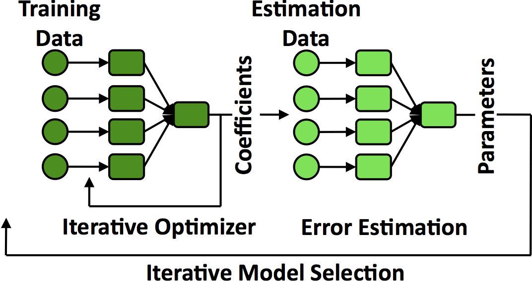Hold-out cross validation method as an example of an iterative method.

How similar are JIT compilers and execution templates?

execution Templates optimize repeated control decisions. In this way, they are similar to a just-in-time (JIT) compiler for the control plane. A JIT compiler transforms blocks of bytecodes into native instructions; execution templates transform blocks of tasks into dependency graphs and other runtime scheduling structures. Table shows the correspondences in this an analogy: an execution template is a function (the granularity JIT compilers typically operate on), a task from the driver to the controller is a bytecode instruction, and a task executing on the worker is a native instruction.

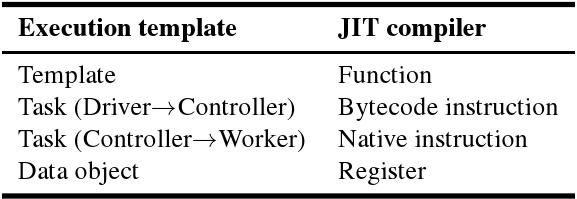Analogy between execution templates and JIT compilers.

Why is Scala implementation of gradient operation 50x slower than C++?

We wrote gradient computation both in C++ and Scala under Spark. Figure shows the result of operation over 64MB of input data. C++ is almost 51 time faster than Scala. We were also shocked by these numbers; to determine the cause of this slowdown, we decompiled the JVM bytecodes Scala generated into Java, rewrote this code to remove its overheads step by step, and recompiled it. The poor performance has three major causes. First, since Scala's generic methods cannot use primitive types (e.g., they must use the Double class rather than a double), every generic method call allocates a new object for the value, boxes the value in it, un-boxes for the operation, and deallocates the object. In addition to cost of a malloc and free, this results in millions of tiny objects for the garbage collector to process. 85\% of logistic regression's CPU cycles are spent boxing/un-boxing. Second, Spark's resilient distributed datasets (RDDs) forces methods to allocate new arrays, write into them, and discard the source array. For example, a map method that increments a field in a dataset cannot perform the increment in-place and must instead create a whole new dataset. This data duplication adds an additional factor of ~2x slowdown. Third, using the Java Virtual Machine has an additional factor of ~3x slowdown over C++. This result is in line with prior studies, which have reported 1.9x-3.7x for computationally dense codes[ Loop Recognition in C++/Java/Go/Scala, A Java vs. C++ performance evaluation: a 3D modeling benchmark ]. In total, this results in Spark code running 51 times slower than C++.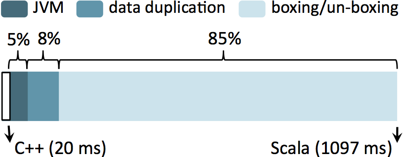

Running gradient operation over 64MB of samples in C++ and Scala. The overhead of Scala is decomposed in to three factors.

What if other frameworks run tasks at the speed of C++?

Nimbus runs common benchmarks (e.g. Logistic Regression shown in the Figure) faster than Naiad and Spark by a factor of 16-43. The speed up comes from two major points 1) efficient tasks in C++, and 2) optimized control plane with execution templates. To disambiguate the two, we also considered the case where Spark and Naiad run optimized code. Spark-opt and Naiad-opt in the Figure show the case where task computations are replaced by a spin-wait as long as C++ tasks. The results show that when available frameworks run optimized tasks, control plane becomes a bottleneck such that even running at scales bigger than 20 workers slows the completion time. Execution templates bring another factor of 4-8 back on the table by removing the runtime overhead.

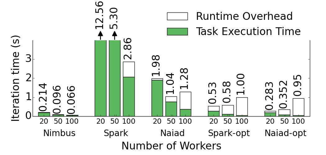Logistic Regression in various frameworks at different scales.

How does Nimbus's task throughput scale?

If the number of workers is W and the number of cores per workers is C then, the runtime overhead of Spark would be O(CW). Thgis is because the centralized controller schedules each task individually and coordinates the reduction and group operations centrally. In case of Naiad the runtime overhead is O(W ²) due to all-to-all synchronization pattern among the nodes. Naiad is a distributed frameworks, and the distributed tracking protocol for timely data flows requires the expensive synchronization for global operations. Specially there is a big constant factor in the big O notation for Naiad, as the overhead depends on the size of the exchanged messages/data required for synchronizations. In case of Nimbus the overhead is O(W), with a small constant factor. Controller only instantiates the templates on the workers with small set of parameters. This allows the Nimbus Tasks throughput scale almost linearly with the number of workers as depicted in the Figure.

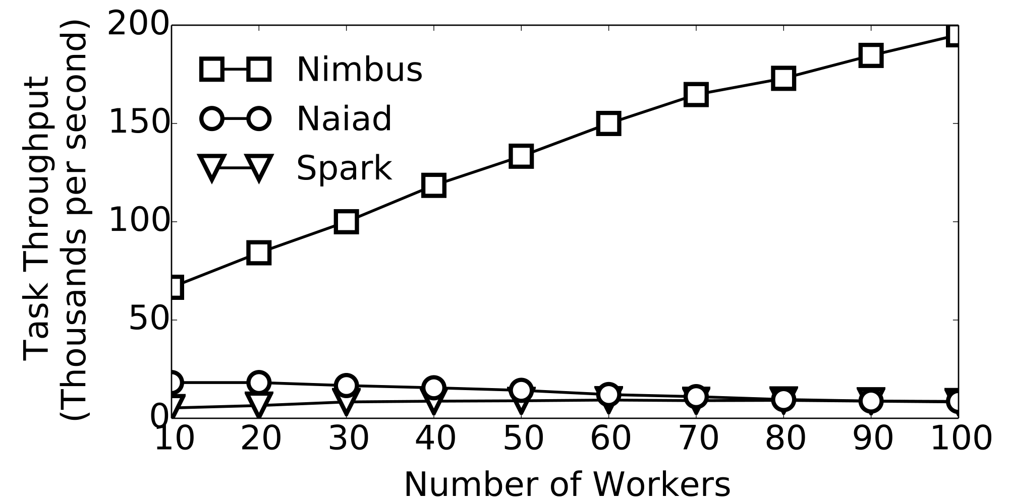Task throughput of various frameworks at scale.

What is the task length distribution of physical simulations?

Physical simulations are good examples for the applications that are written to run fast, instead of fitting the constraints of frameworks. Scientist and programmers are instantly trying to run bigger simulations with more accuracy and no waste of resources in terms of CPU cycles or Memory is acceptable. PhysBAM is a Physics based simulations library. The Figure shows the CDF of the task length in water simulation. It is a canonical fluid simulations with both particles and grid-based operations. The simulations includes 26 stages of computations, over more than 40 different type of variables. For the experiment we used a 256³ with more than 9GB of in-memorry variables. The median task length is 13ms, while there are tasks as short as 100us.

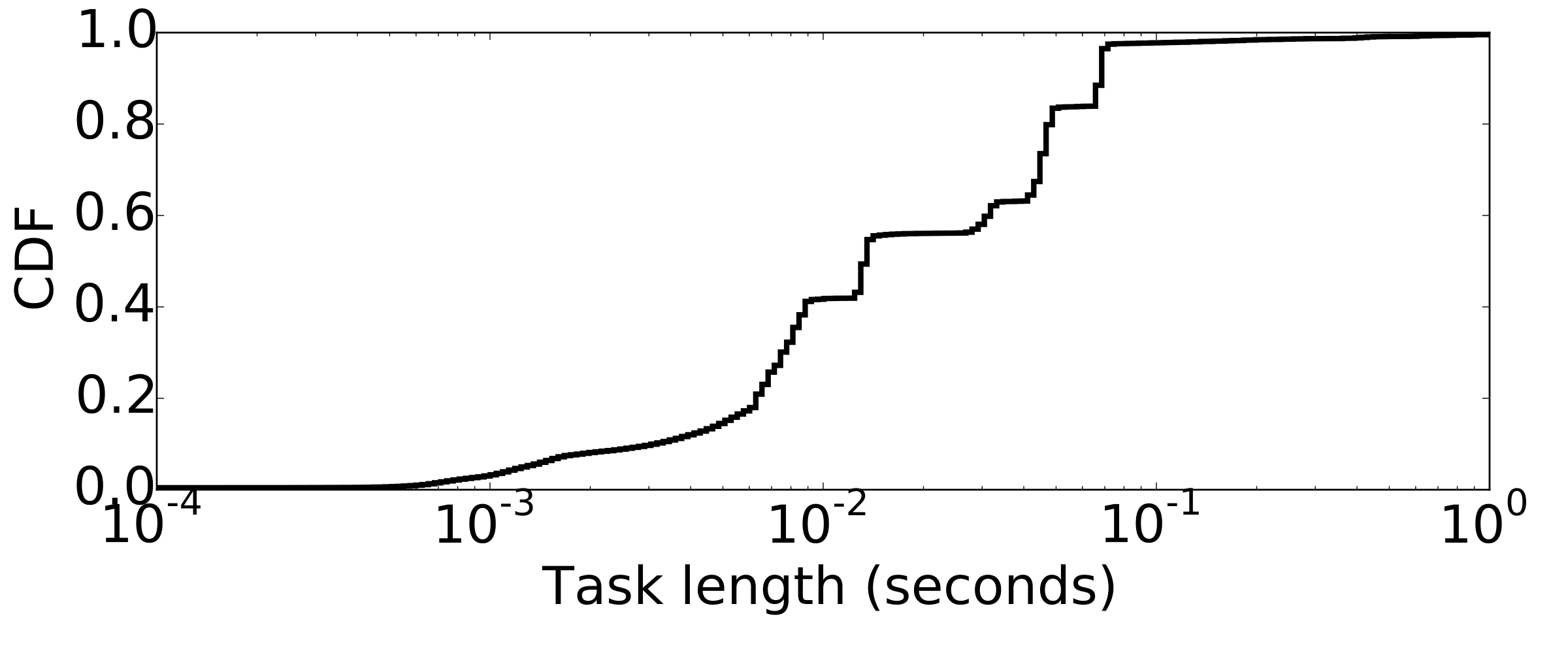Task length distribution of water simulation from PhysBAM library.